Dynamic Communities detection and evaluation

If tnerwork library is not installed, you need to install it, for instance using the following command

#%%capture #avoid printing output
#!pip install --upgrade git+https://github.com/Yquetzal/tnetwork.git

%load_ext autoreload
%autoreload 2
import tnetwork as tn
import seaborn as sns
import pandas as pd
import networkx as nx
import numpy as np

Creating an example dynamic graph with changing community structure

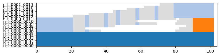
We create a simple example of dynamic community evolution using the generator provided in the library. We generate a simple ship of Theseus scenario. Report to the corresponding tutorial to fully understand the generation part if needed.

my_scenario = tn.ComScenario(alpha=0.8,random_noise=0.1)
[com1,com2] = my_scenario.INITIALIZE([6,6],["c1","c2"])
(com2,com3)=my_scenario.THESEUS(com2,delay=20)
my_scenario.CONTINUE(com3,delay=10)

#visualization
(generated_network_IG,generated_comunities_IG) = my_scenario.run()

plot = tn.plot_longitudinal(generated_network_IG,generated_comunities_IG,height=200)
generated_network_SN = generated_network_IG.to_DynGraphSN(slices=1)
generated_communities_SN = generated_comunities_IG.to_DynCommunitiesSN(slices=1)

100% (8 of 8) |##########################| Elapsed Time: 0:00:00 ETA:  00:00:00/usr/local/lib/python3.7/site-packages/numpy/core/numeric.py:2327: FutureWarning: elementwise comparison failed; returning scalar instead, but in the future will perform elementwise comparison
  return bool(asarray(a1 == a2).all())

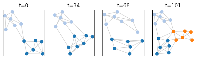
Let’s look at the graph at different stages. There are no communities.

last_time = generated_network_IG.end()
print(last_time)
times_to_plot = [0,int(last_time/3),int(last_time/3*2),last_time-1]
plot = tn.plot_as_graph(generated_network_IG,ts=times_to_plot,width=200,height=200)

102

Algorithms for community detection are located in the tnetwork.DCD package

import tnetwork.DCD as DCD

First algorithm: Iterative match

Iterative match consists in applying a static algorithm at each step and matching communities in successive snapshots if they are similar. Check the doc for more details.

Without particular parameters, it uses the louvain method and the jaccard coefficient.

com_iterative = DCD.iterative_match(generated_network_SN)

The static algorithm, the similarity function and the threashold to consider similar can be changed

custom_match_function = lambda x,y: len(x&y)/max(len(x),len(y))
com_custom = DCD.iterative_match(generated_network_SN,match_function=custom_match_function,CDalgo=nx.community.greedy_modularity_communities,threshold=0.5)

Visualizing communities

One way to visualize the evolution of communities is to plot the graph at some snapshots. By calling the plot_as_graph function with several timestamps, we plot graphs at those timestamps while ensuring:

• That the position of nodes stay the same between snapshots
• That the same color in different plots means that nodes belong to the same dynamic communities

last_time = generated_network_IG.end()
times_to_plot = [0,int(last_time/3),int(last_time/3*2),last_time-1]
plot = tn.plot_as_graph(generated_network_IG,com_iterative,ts=times_to_plot,auto_show=True,width=200,height=200)

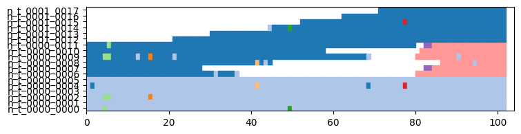
Another solution is to plot a longitudinal visualization: each horizontal line corresponds to a node, time is on the x axis, and colors correspond to communities. Grey means that a node corresponds to no community, white that the node is not present in the graph (or has no edges)

to_plot = tn.plot_longitudinal(generated_network_SN,com_iterative,height=200)

Survival Graph

This method matches communities not only between successive snaphsots, but between any snapshot, constituting a survival graph on which a community detection algorithm detects communities of communities => Dynamic communities

com_survival = DCD.label_smoothing(generated_network_SN)
plot = tn.plot_longitudinal(generated_network_SN,com_survival,height=200)

starting label_smoothing method

Smoothed louvain

The smoothed Louvain algorihm is very similar to the simple iterative match, at the difference that, at each step, it initializes the partition of the Louvain algorithm with the previous partition instead of having each node in its own community as in usual Louvain.

It has the same options as iterative match, since only the community detection process at each step changes, not the matching

com_smoothed = DCD.smoothed_louvain(generated_network_SN)
plot = tn.plot_longitudinal(generated_network_SN,com_smoothed,height=200)

 98% (100 of 102) |##################### | Elapsed Time: 0:00:00 ETA:   0:00:00

Smoothed graph

The smoothed-graph algorithm is similar to the previous ones, but the graph at each step is smoothed by the community structure found in the previous step. (An edge with a small weight is added between any pair of nodes that where in the same community previously. This weight is determined by a parameter alpha)

com_smoothed_graph = DCD.smoothed_graph(generated_network_SN)
plot = tn.plot_longitudinal(generated_network_SN,com_smoothed_graph,height=200)

 97% (99 of 102) |###################### | Elapsed Time: 0:00:00 ETA:   0:00:00

Matching with a custom function

The iterative match and survival graph methods can also be instantiated with any custom community detection algorithm at each step, and any matching function, as we can see below. The match function takes as input the list of nodes of both communities, while the community algorithm must follow the signature of networkx community detection algorithms

custom_match_function = lambda x,y: len(x&y)/max(len(x),len(y))
com_custom2 = DCD.iterative_match(generated_network_SN,match_function=custom_match_function,CDalgo=nx.community.greedy_modularity_communities)
plot = tn.plot_longitudinal(generated_network_SN,com_custom2,height=200)

Another algoritm in python: CPM

CPM stands for Clique Percolation Method. An originality of this approach is that it yiealds overlapping communities.

Be careful, the visualization is not currently adapted to overlapping clusters…

com_CPM = DCD.rollingCPM(generated_network_SN,k=3)
plot = tn.plot_longitudinal(generated_network_SN,com_CPM,height=200)

CD detection done 102

Dynamic partition evaluation

The goal of this section is to present the different types of dynamic community evalutation implemented in tnetwork.

For all evaluations below, no conclusion should be drawn about the quality of algorithms… .

#Visualization
plot = tn.plot_longitudinal(communities=generated_comunities_IG,height=200,sn_duration=1)

Quality at each step

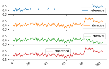
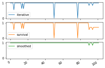
The first type of evaluation we can do is simply to compute, at each type, a quality measure. By default, the method uses Modularity, but one can provide to the function its favorite quality function instead. It is the simplest adaptation of internal evaluation.

Note that * The result of an iterative approach is identical to the result of simply applying a static algorithm at each step * Smoothing therefore tends to lesser the scores. * The result migth or might not be computable at each step depending on the quality function used (e.g., modularity requires a complete partition of the networks to be computed)

quality_ref,sizes_ref = DCD.quality_at_each_step(generated_communities_SN,generated_network_SN)
quality_iter,sizes_iter = DCD.quality_at_each_step(com_iterative,generated_network_SN)
quality_survival,sizes_survival = DCD.quality_at_each_step(com_survival,generated_network_SN)
quality_smoothed,sizes_smoothed = DCD.quality_at_each_step(com_smoothed,generated_network_SN)

df = pd.DataFrame({"reference":quality_ref,"iterative":quality_iter,"survival":quality_survival,"smoothed":quality_smoothed})
df.plot(subplots=True,sharey=True)

array([<matplotlib.axes._subplots.AxesSubplot object at 0x11f1bd8d0>,
       <matplotlib.axes._subplots.AxesSubplot object at 0x11f5aa6d0>,
       <matplotlib.axes._subplots.AxesSubplot object at 0x11e993e10>,
       <matplotlib.axes._subplots.AxesSubplot object at 0x108343d10>],
      dtype=object)

Average values

One can of course compute average values over all steps. Be careful however when interpreting such values, as there are many potential biases: * Some scores (such as modularity) are not comparable between graphs of different sizes/density, so averaging values obtained on different timesteps might be incorrect * The clarity of the community structure might not be homogeneous, and your score might end up depending mostly on results on a specific period * Since the number of nodes change in every step, we have the choice of weighting the values by the size of the network * etc.

Since the process is the same for all later functions, we won’t repeat it for the others in this tutorial

print("iterative=", np.average(quality_iter),"weighted:", np.average(quality_iter,weights=sizes_iter))
print("survival=", np.average(quality_survival),"weighted:", np.average(quality_survival,weights=sizes_survival))
print("smoothed=", np.average(quality_smoothed),"weighted:", np.average(quality_smoothed,weights=sizes_smoothed))

iterative= 0.4289862014179952 weighted: 0.4357461539951767
survival= 0.39927872978552464 weighted: 0.39689292217118277
smoothed= 0.42992554634769103 weighted: 0.4365993079467363

Similarity at each step

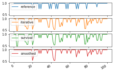
A second type of evaluation consists in adaptating external evaluation, i.e., comparison with a known reference truth.

It simply computes at each step the similarity between the computed communities and the ground truth. By default, the function uses the Adjusted Mutual Information (AMI or aNMI), but again, any similarity measure can be provided to the function.

Note that, as for quality at each step, smoothing is not an advantage, community identities accross steps has no impact.

There is a subtility here: since, often, the dynamic ground truth might have some nodes without affiliations, we make the choice of comparing only what is known in the ground truth, i.e., if only 5 nodes out of 10 have a community in the ground truth at time t, the score of the proposed solution will depends only on those 5 nodes, and the affiliations of the 5 others is ignored

quality_iter,sizes = DCD.similarity_at_each_step(generated_communities_SN,com_iterative)
quality_survival,sizes = DCD.similarity_at_each_step(generated_communities_SN,com_survival)
quality_smoothed,sizes = DCD.similarity_at_each_step(generated_communities_SN,com_smoothed)

df = pd.DataFrame({"iterative":quality_iter,"survival":quality_survival,"smoothed":quality_smoothed})
df.plot(subplots=True,sharey=True)

array([<matplotlib.axes._subplots.AxesSubplot object at 0x11fb59290>,
       <matplotlib.axes._subplots.AxesSubplot object at 0x11f90ccd0>,
       <matplotlib.axes._subplots.AxesSubplot object at 0x11eb31c50>],
      dtype=object)

Smoothness Evaluation

We can evaluate the smoothness of a partition by comparing how the partition in each step is similar to the partition in the next. Again, any measure can be used, by default the overlapping NMI, because two adjacent partitions do not necessarily have the same nodes. * This evaluation is internal. * This time, it depends on the labels given to nodes accross steps, so a static algorithm applied at each step would have a score of zero. * The score does not depends at all on the quality of the solution, i.e., having all nodes in the same partition at every step would obtain a perfect score of 1

quality_ref,sizes_ref = DCD.consecutive_sn_similarity(generated_communities_SN)
quality_iter,sizes_iter = DCD.consecutive_sn_similarity(com_iterative)
quality_survival,sizes_survival = DCD.consecutive_sn_similarity(com_survival)
quality_smoothed,sizes_smoothed = DCD.consecutive_sn_similarity(com_smoothed)

df = pd.DataFrame({"reference":quality_ref,"iterative":quality_iter,"survival":quality_survival,"smoothed":quality_smoothed})
df.plot(subplots=True,sharey=True)

array([<matplotlib.axes._subplots.AxesSubplot object at 0x11f103850>,
       <matplotlib.axes._subplots.AxesSubplot object at 0x11c7af710>,
       <matplotlib.axes._subplots.AxesSubplot object at 0x11fc5c7d0>,
       <matplotlib.axes._subplots.AxesSubplot object at 0x11f46e610>],
      dtype=object)

Global scores

Another family of scores we can compute are not based on step by step computations, but rather compute directly a single score on whole communities

Longitudinal Similarity

This score is computed using a usual similarity measure, by default the AMI. But instead of computing the score for each step independently, it is computed once, consider each (node,time) pair as a data point (instead of each node in a static network). * The evaluation is external, it requires a (longitudinal) reference partition * It takes into account both the similarity at each step and the labels accros steps * Similar to step by step similarity, only (node,time) couples with a known affiliation in the reference partition are used, others are ignored

quality_iter = DCD.longitudinal_similarity(generated_communities_SN,com_iterative)
quality_survival = DCD.longitudinal_similarity(generated_communities_SN,com_survival)
quality_smoothed = DCD.longitudinal_similarity(generated_communities_SN,com_smoothed)

print("iterative: ",quality_iter)
print("survival: ",quality_survival)
print("smoothed: ",quality_smoothed)

iterative:  0.9451292907933111
survival:  0.8234124633781458
smoothed:  0.9868504021347683

Global Smoothness

Trhee methods are proposed to evaluate the smoothness at the global level.

The first is the average value of partition smoothness as presented earlier, and is called SM-P for Partition Smoothness

The second one computes how many changes in affiliation there are, and the score SM-N (Node Smoothness) is 1/number of changes * It penalizes methods with many glitches, i.e., transient affiliation change. * It does not penalize long term changes

The third computes instead the entropy per node, and the score SM-L (Label smoothness) is 1/average node entropy. * It does not penalize much glitches * It advantages solutions in which nodes tend to belong to few communities

For all 3 scores, higher is better.

print("iterative: SM-P" ,DCD.SM_P(com_iterative), "SM-N:",DCD.SM_N(com_iterative), " SM-L:",DCD.SM_L(com_iterative))
print("survival: SM-P ",DCD.SM_P(com_survival), "SM-N:",DCD.SM_N(com_survival), " SM-L:",DCD.SM_L(com_survival))
print("smoothed: SM-P:",DCD.SM_P(com_smoothed), "SM-N:",DCD.SM_N(com_smoothed), " SM-L:",DCD.SM_L(com_smoothed))

iterative: SM-P 0.9001839896381273 SM-N: 0.023255813953488372  SM-L: 3.6914110221883676
survival: SM-P  0.9026384453495243 SM-N: 0.03333333333333333  SM-L: 18.48733611718878
smoothed: SM-P: 0.9470754696907387 SM-N: 0.05555555555555555  SM-L: 4.416478672484498